Linear Data Structures: Sequential Organization
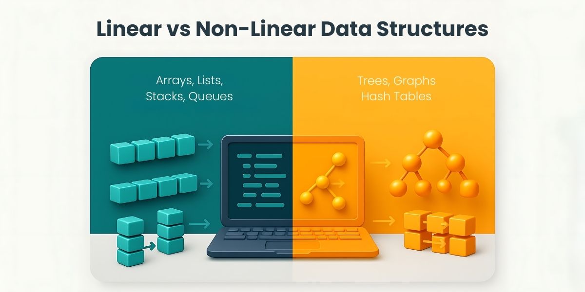
Linear data structures arrange elements in a sequence. Common examples include arrays, linked lists, stacks, and queues. All these structures are essentially one-dimensional lines of data (conceptually), but their implementations differ.
Arrays The Foundation
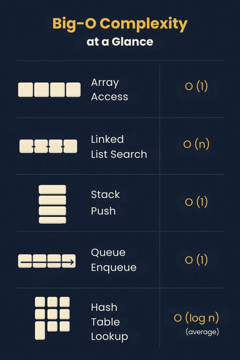
In lowlevelstatic arrays (e.g., C/Java), elements share a fixed type and contiguous memory; high-level dynamic arrays (e.g., Python lists) can hold mixed types and resize automatically. The key advantage of arrays is direct access: retrieving or updating the i-th element takes constant time (O(1)). Arrays are the foundation for other fundamental data structures.
However, arrays have fixed size (in static languages) or need dynamic resizing (in high-level languages). Inserting or deleting an element in the middle of an array typically requires shifting many elements (O(n) time). In programming, dynamic arrays handle resizing under the hood, giving amortized O(1) for appending.
Arrays typically benefit from CPU cache locality; linked lists suffer from pointer chasing, which can make them slower in practice even when asymptotic costs look similar.
# Example: Array in Python
arr = [10, 20, 30, 40] # A list of 4 elements
print(arr[2]) # Access index 2: outputs 30 (constant time)
arr.append(50) # Add element at end (amortized O(1))
arr.insert(1, 15) # Insert at index 1 (O(n) time, shifts elements)
Use cases: Arrays are ubiquitous in scientific computing (for matrices, images, sensor data). They power numerical libraries (e.g., NumPy), graph algorithms (adjacency matrices). Arrays are among the oldest and most important data structures, used by almost every program.
Linked Lists: Dynamic and Flexible
A linked list is a chain of nodes connected by pointers (or references). Each node typically contains data and a pointer to the next node (and possibly to the previous node in a doubly linked list). The list can grow or shrink dynamically without preallocating memory.
The classic singly linked list allows quick insertion or deletion at the head (O(1) time), whereas insertion/deletion in an array can be expensive. Unlike arrays, linked lists do not provide constant-time random access. To find the i-th element, you must traverse the list from the head (O(n) time). Also, each node requires extra memory for the pointer.
Linked lists are beneficial when your program needs frequent insertions/deletions from the list (e.g., implementing other data structures like stacks, queues, or adjacency lists for graphs). They allow O(1) insertion/deletion at known positions (e.g., head/tail); arbitrary positions still require O(n) traversal.
Types:
Singly linked list: each node points to the next
Doubly linked list: nodes have next and previous pointers (useful for two-way traversal and easy deletion)
Circular linked list: the last node points back to the head (can be useful for round-robin scheduling)
# Example: Linked List insertion in Python-like pseudo-code
class Node:
def __init__(self, data):
self.data = data
self.next = None
# Insert new node with value 10 at head of list
new_node = Node(10)
new_node.next = head # head is the current first node
head = new_node
Here, inserting at the head took constant time (O(1)) by just changing pointers.
Use cases: Linked lists are often used to implement stacks and queues, adjacency lists in graph algorithms, and undo/redo buffers. In memory management, free blocks are sometimes tracked via a linked list. Mastering linked lists helps you understand dynamic memory usage and pointer arithmetic.
Stacks: Last-In, First-Out (LIFO)
A stack follows Last-In, First-Out (LIFO) order: the last element added is the first one removed. Think of a stack of plates; you add and remove plates from the top. The two primary operations are push (add to top) and pop (remove from top). Both operations run in constant time (O(1)).
Internally, a stack can be implemented using an array (with an index for the top) or a linked list (inserting/removing at the head).
# Example: Python list as stack
stack = [ ]
stack.append('apple') # push 'apple'
stack.append('banana') # push 'banana'
top = stack.pop() # pop returns 'banana'
print(top, len(stack)) # outputs: banana 1
Applications: Stacks appear everywhere: function call stacks (where the return address is pushed/popped), expression evaluation (parsing and compilers), undo functionality in text editors, and backtracking algorithms (like depth-first search). Because of its simplicity, stack operations are trivially efficient, but choosing a stack makes sense when LIFO ordering is required.
Queues: First-In, First-Out (FIFO)
A queue follows First-In, First-Out (FIFO) order: the first element added is the first one removed. Common operations are enqueue (add to tail) and dequeue (remove from head). Simple queues can be implemented using linked lists or circular arrays. Both enqueue and dequeue run in constant time (O(1)) if implemented well.
Variants:
Simple Queue: like a line of people waiting; use a circular array (ring buffer) or a linked list with head/tail; in Python, prefer collections.deque (O(1) enqueue/dequeue)
Circular Queue: uses an array with wrap-around to maximize space usage
Priority Queue: not strictly FIFO; elements have priorities and the highest-priority element is removed first (often implemented with a binary heap)
# Example: Python deque for queue
from collections import deque
queue = deque()
queue.append('task1') # enqueue 'task1'
queue.append('task2') # enqueue 'task2'
first = queue.popleft() # dequeue (FIFO) -> 'task1'
print(first, len(queue)) # outputs: task1 1
Applications: Queues are everywhere in engineering: printer spooling, CPU process scheduling, network packet handling, breadth-first search in graphs, and event handling systems. The real-world metaphor is like a line in a bank; it ensures fairness (the oldest request gets served first).
Non-Linear Data Structures: Complex Relationships
Linear data structures are not always sufficient. Non-linear data structures allow items to be related in more complex ways. The most common non-linear structures are trees and graphs, which model hierarchical and network relationships, respectively.
Trees: Hierarchical Structures
A tree is a hierarchical data structure composed of nodes connected by edges, with one node designated as the root. Each node can have zero or more child nodes. A node with no children is called a leaf. Trees impose a parent-child hierarchy, unlike linear lists. Strictly speaking, you can think of lists as a special form of Trees.
One of the simplest and most famous examples is the binary tree, where each node has at most two children (commonly labeled left and right). A Binary Tree Data Structure is a hierarchical data structure in which each node has at most two children.
Basic operations: Common tree operations include insertion, deletion, and traversals (e.g., in-order, pre-order, post-order for binary trees). In a binary search tree (BST)---a binary tree with a sorting invariant---each left subtree has values less than the parent, and each right subtree has greater values. This property allows searching in O(h) time, where h is the tree height (for a balanced tree h≈log n).
Self-balancing trees: Regular BSTs can become skewed (like a linked list) if data is inserted in sorted order. To guarantee efficiency, self-balancing variants exist (e.g., AVL trees, Red-Black trees). These restructure themselves (via rotations) to keep height ~O(log n). This yields O(log n) search, insert, and delete. In practice, many language libraries use balanced trees for sorted sets/maps.
Applications: Trees appear in file systems (directories and files form a tree), HTML/DOM structure (web pages), decision trees (AI/ML), and expression parsing (compilers use parse trees or abstract syntax trees). They are also fundamental in databases (B/B+-trees index data on disk) and in networking (prefix tries for IP lookup).
Because they mirror hierarchical relationships, trees are useful anytime data naturally branches---from modeling organizational structures to representing decision-making processes in business applications.
Graphs: Interconnected Networks
A graph is a set of vertices (nodes) connected by edges, representing one of the most versatile non-linear data structures. Graphs can be undirected (edges have no direction) or directed (edges are arrows). Unlike trees, graphs can have cycles and complex connectivity. Mathematically speaking, trees are special cases of graphs.
Representation:
Adjacency List: For each vertex, store a list of its neighbors. Good for sparse graphs (space O(V+E))
Adjacency Matrix: For unweighted graphs, matrix[i][j] is 1/0 for edge/no edge; for weighted graphs, matrix[i][j] stores the edge weight (with 0/∞/None as the 'no edge' sentinel). Fast lookup but uses O(V²) space, so best for dense graphs.
Traversal: Key algorithms include Breadth-First Search (BFS) and Depth-First Search (DFS). BFS explores neighbors level by level and can find shortest paths in unweighted graphs. DFS goes deep along a branch and is useful for detecting cycles and for topological sort on DAGs. Shortest-path algorithms (e.g., Dijkstra for non-negative weights; Bellman-Ford when negative edges may exist) find optimal routes.
Real-world usage: Social networks are prime examples of graphs: users are nodes, friendships are edges. Graph algorithms power friend recommendations and community detection. Transport networks (roads, air routes) are graphs---GPS apps find shortest driving routes using graph search. Even the web itself is a giant directed graph of hyperlinks.
In the MENA context, graphs model everything from Cairo's metro system to Saudi Arabia's planned intercity transport networks.
Hash Tables: Fast Lookups
A hash table (or hash map/dictionary) implements an associative array---a collection of key-value pairs---with very fast lookup. It uses a hash function to convert each key into an index of an underlying array. Ideally, the hash function distributes keys uniformly, so that most indices are used evenly.
When you insert a key, you compute its hash and place it at that index; when you look up a key, you compute its hash to find its value. Collisions (two keys hashing to the same index) are handled by techniques like chaining (each index holds a linked list of entries) or open addressing (probe for an empty slot).
With a good hash function and a bounded load factor (via rehashing), insert, delete, and lookup are average-case O(1) but worst-case O(n) under heavy collisions.
Applications: Hash tables are everywhere: dictionaries in programming languages, some database systems' hash indexes for specific workloads, caching, symbol tables in compilers, and even caching DNS entries on the internet. Their speed makes them ideal for tasks like counting word frequencies in text, managing user sessions, or any situation requiring quick lookup by key.
The trade-off is memory overhead (and care in choosing a good hash function), but the payoff is extremely fast access---critical for real-time applications.
Data Structures in Action: Real-World Applications & Case Studies
Applications Across STEM Disciplines
Fundamental data structures form the backbone of many STEM applications:
Scientific Computing: Arrays and matrices (implemented as arrays) are fundamental. Linear algebra libraries rely on contiguous arrays for vector/matrix operations. Sparse matrices and graphs represent networks in physics or engineering simulations.
Data Science & Machine Learning: High-volume data requires efficient storage and processing. Pandas and NumPy use arrays under the hood. Hash tables (dictionaries) are used in feature extraction (word counts), and trees are the basis of decision-tree models and random forests. Efficient algorithms for sorting, searching, and indexing data are crucial for data analysis.
Operating Systems and Databases: OS schedulers use queues (ready queue) and stacks (call stack). Filesystems use trees to index directories. Most databases use B/B+-trees for on-disk indexes; some engines also provide hash indexes for specific equality-lookup workloads.
Algorithms and Research: Areas like cryptography, bioinformatics, and robotics rely on complex data structures. For example, genome sequences might be handled as suffix trees; robot motion planning can use graphs of possible states; cryptographic algorithms use trees and graphs in key management.
Data structures and algorithms are fundamental in almost every area of software development, including operating systems, databases, machine learning, and social networks. Whether building a simple calculator or simulating weather patterns, these structures determine how efficiently you can solve the problem.
MENA-Specific Case Studies
In Egypt, Saudi Arabia, and the broader Middle East and North Africa region, several digital transformation initiatives highlight the growing need for computational skills: